The team

We are three graduate students in the Astronomy Department at Harvard University.
This is our final project for CS205: Computing Foundations for Computational Science.

BEHALF at a Glance

BEHALF is a parallel Barnes-Hut algorithm for solving the N-body problem, using MPI and GPU computing. This code was build for the final project of the CS205 class at Harvard in the Spring 2018 semester.

Keep exploring our website to learn more about the N-body problem, our parallel implementation of the Barnes-Hut algorithm, and our results simulating an elliptical galaxy.

Explore different components of our project
or keep scrolling to see it all!

  • Introduction:
    N-body problem

    The N-body problem refers to the challenge of predicting the motion of N individual objects under the force of gravity. A typical example consists of evolving the motion of stars or dark matter particles in a galaxy.

  • Barnes-Hut and
    Oct-Trees

    Barnes-Hut is a tree algorithm that can greatly speed-up the N-body computation by hierarchically subdividing space into octants, until there will be at most one particle per cell, and approximating the gravitational force between objects very far away from each other.

  • Code Implementation

    Here we describe our octree implementation, leapfrog integration, and parallel approach for the Barnes-Hut algorithm. All the code can be found at our GitHub repo.

  • Performance and Analysis

    In this section, we analyze the accuracy of our method and the parallel performance of our code (e.g., speed-up, efficiency, weak and strong scaling).

  • Movies

    Finally, we present movies of the galaxies we simulated using BEHALF.

Introduction: N-Body Problem

The N-body problem broadly describes the problem of predicting the future trajectories of a group of objects under the mutual gravitational forces they exert on one another, given each individual object's current position and velocity. The first general formulation of the N-body problem was proposed by Newton when he was studying the motions of Jupiter and its moons (Newton 1687). In Astronomy, the N-body problem has been studied at a wide variety of scales: ranging from the study of asteroids near Jupiter (Brož et al. 2008) to the study of the largest gravitationally bound clusters in the Universe (Angulo et al. 2012).

For our project, we will be focusing on an intermediate regime: the evolution of galaxies. The fundamental resolution unit in the study of galaxies is a star; stars are born out of the cold and dense gas inside the galaxy, and they move around the galaxy due to the forces exerted by hundreds of billions of other stars in the galaxy halo. Consequently, studying how galaxies form and evolve is a rich and complicated endeavor that can no longer be fully modeled using just analytical theory. The dynamic scale that needs to be resolved in order to self-consistently study galaxies is enormous and spans many orders of magnitudes, necessitating the use of high performance computing and sophisticated codes that can utilize various different HPC programming models.

Naively, the N-body problem can be solved by considering all pairs of individual points and adding up the contributions from all such particle-particle interactions. Nonetheless, this approach scales quadratically with the number of particles N: the running time is O(\(N^2\)). Most realistic galaxy simulations require upwards of hundreds of millions of resolution elements. The \(N^2\) scaling of the naive approach would make computations at that scale simply not feasible. Consequently, astronomers have come up with various approximate methods to calculate the forces in the N-body problem, such as tree-based methods (Barnes and Hut 1986) and particle mesh methods (Darden et al. 1993). For our project, we will be focusing on parallelizing the Barnes-Hut (BH) algorithm.

The Barnes-Hut Algorithm


The BH algorithm and various modifications of the original algorithm have been extensively used in astrophysical simulations (e.g., Katz et al. 1995, Wadsley et al. 2004, Springel et al. 2005 ). The fundamental assumption in all variants of the BH algorithm is that the gravitational pull of many far-away bodies can be approximated by replacing the group of many distant bodies with a single object located at the center of mass and encompassing the total mass of those bodies (Barnes and Hut 1986).

Barnes and Hut represented this idea using the Octree data structure. In octrees, each internal node has exactly eight child nodes. Octrees have been used in various domains to partition a three-dimensional space by recursively subdividing the space into octants. The figure shown below is an illustration of the 2-dimensional version of the same problem using quadtrees instead of octrees. The upper right quadrant has been recursively subdivided into 4 nodes at each level, until each leaf in the tree contains at most one particle. In this example, we needed 4 levels in the tree in order to fully subdivide the upper right quadrant.

By grouping distant particles together, the far-field approximation requires significantly fewer floating point operations than the naive force calculation. Barnes and Hut found that this approach scales as O(N log N), where the tree traversal takes roughly log(N) operations and calculating the force for the N particles in the system requires N operations.

We will exemplify this by computing the force exerted on the particle highlighted in red in the upper right corner. Particles in orange squares are sufficiently far away from the target particle that we can group them based on their center of mass and apply the far-field force approximation. However, the green particle is sufficiently close to the target particle such that we will instead compute the precise gravitational force exerted by this particle. In total, Barnes-Hut required only 5 force calculations instead of 23 using the exact particle-particle force calculations.

Code Implementation


To download, install, and run the BEHALF package, see the Github Source Repository.


Octree

There are two main algorithms required for the force calculation using an octree: (1) building the tree and (2) traversing the tree to calculate the force on a single body. The pseudocode for these two algorithms is presented below.

 function insertParticle(particle, node)
		if(particle.position is not in node.box): # if particle is not in node's
		bounding box return # end function if(node has no particles):
				node.particle = particle #
			particle is now assigned to node if(node is an internal node):
			updateCenterOfMass(node) # update center of mass of node
			updateTotalMass(node) # update total mass of node for child
			in node.children: insertParticle(particle, child) # insert particle
			into the appropriate child node if(node is an external node): # if node already has another particle
			associated with it createChildren(node) # subdivide this node into its 8 children for child
			in node.children:
			insertParticle(node.particle, child) # insert the existing
			node.particle into the appropriate child node for child in node.children:
			insertParticle(particle, child) # insert particle into the appropriate child node
						

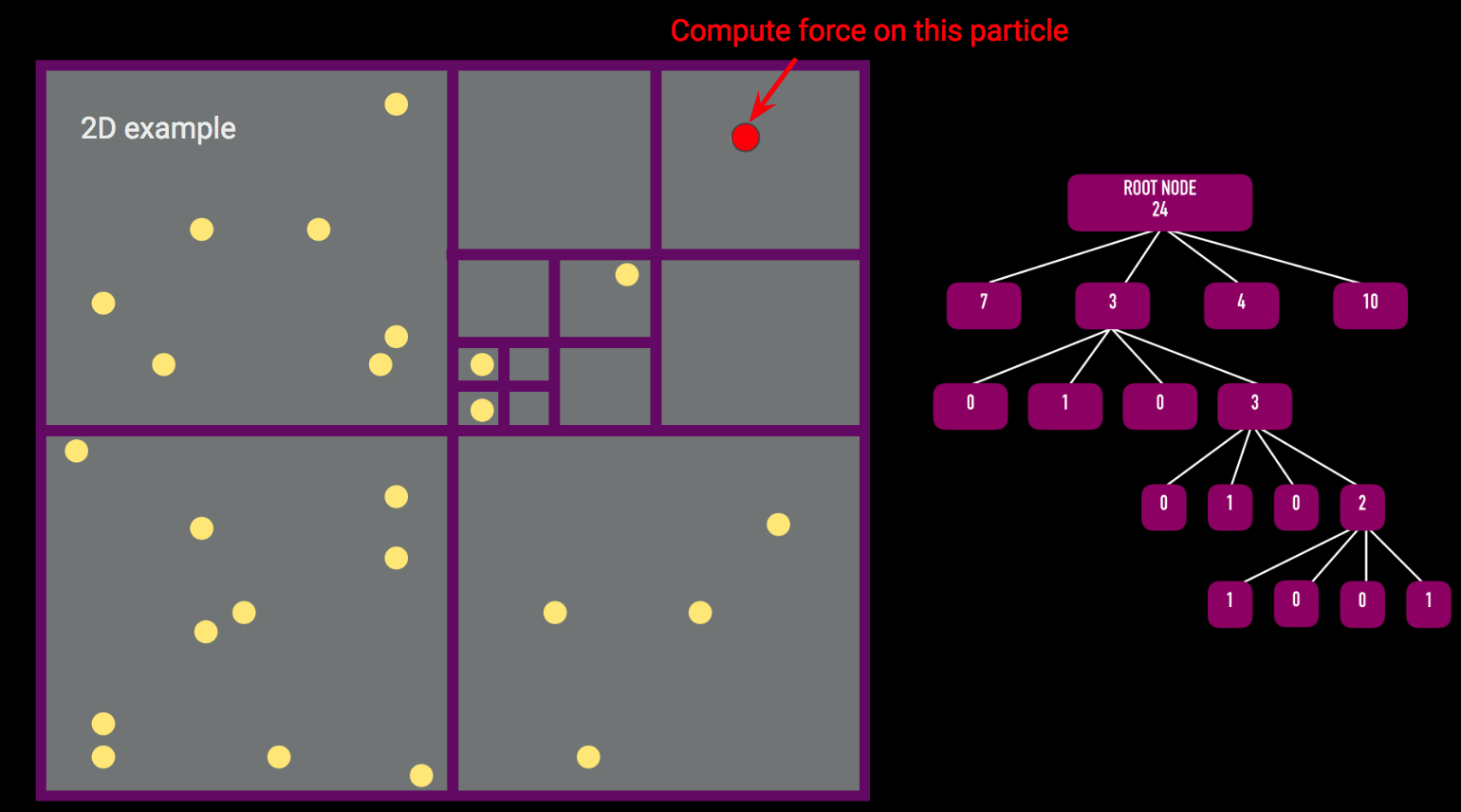
The insertParticle algorithm must be run for every particle in the simulation. The algorithm starts by checking to see if the particle is inside the given node's bounding box. Assuming it is, if the node has no particles, the particle currently being considered will be assigned to the given node. If the node is an internal node (that is, it has child nodes) but has no particles associated with it, we insert the particle into the appropriate child node and update the center of mass and the total mass of the node. If the node is an external node (i.e. it has no children) but already has a particle associated with it, we must first create children for that node and then recursively assign both the particle that was already assigned to the external node and the new particle that we were originally assigning. Once we loop over all particles, each leaf node will have only one particle associated with it.

 function calculateAcceleration(particle, node, thetaTolerance)
		if(node.leaf):
		directAccelCalculation(node.particle, particle) # directly sum this node's
		particle's force on the particle we're considering theta
		= node.size/distance(node.com, particle.position)
		if(theta is less than thetaTolerance):
		farFieldForceCalculation(node.mass, node.com, particle)
		# far field approximation is valid else: # far field approximation is not valid for child in node.chilren:
		calculateAcceleration(particle, child, thetaTolerance)


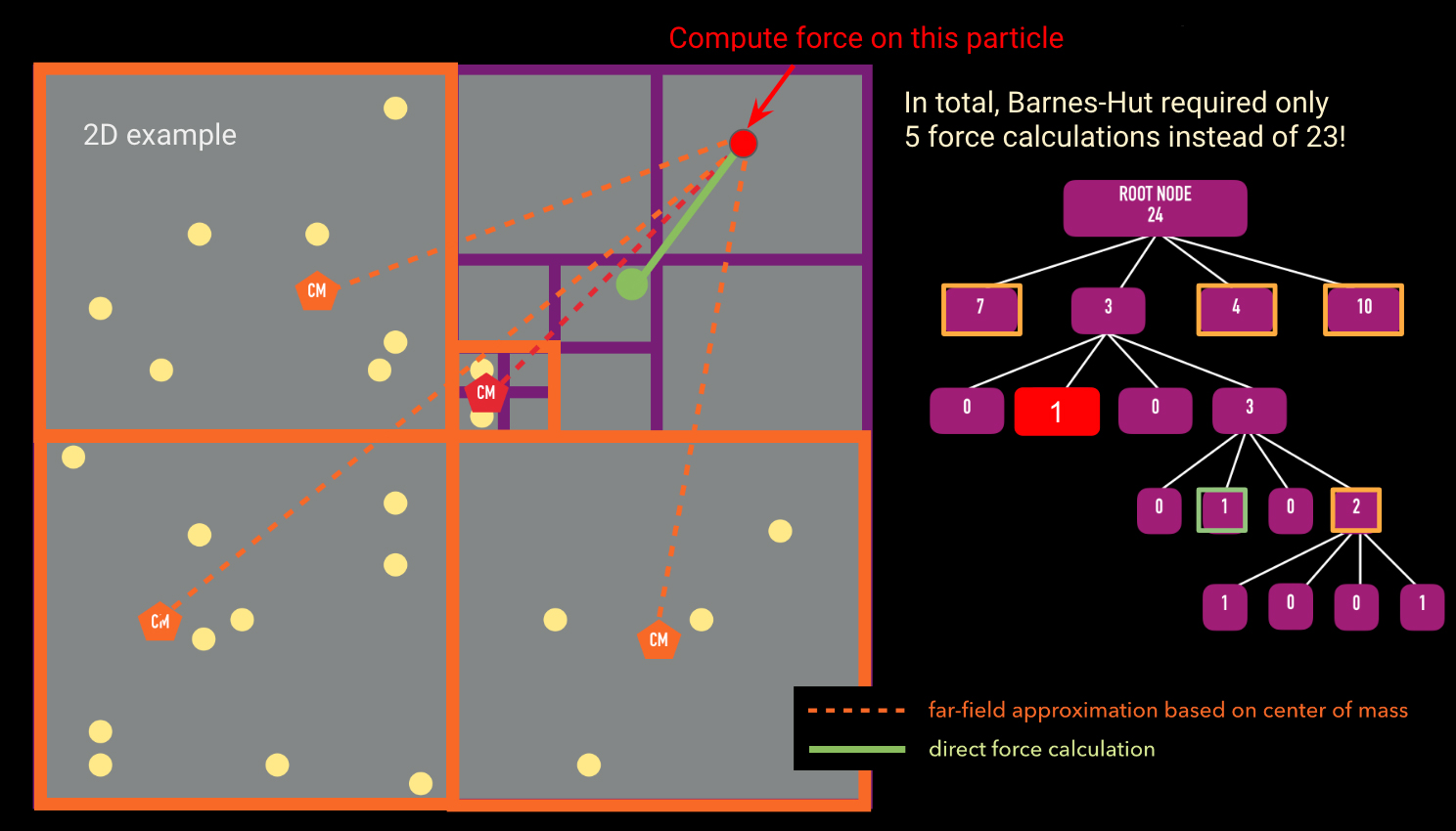
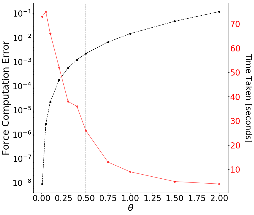
calculateAcceleration takes in the particle we want to calculate the force for, the node we are currently comparing against, and thetaTolerance (the opening angle). The algorithm first starts by checking whether the node we are currently comparing against is a leaf node. If it is, it holds only one particle and we must directly calculate the gravitational influence of this particle on the the particle we passed in as an argument. If the current node is not a leaf, we calculate the opening angle theta (given by the size of the node divided by the distance from the node to the particle). If the opening angle is less than some pre-defined thetaTolerance (most codes in literature use 0.5; Springel et al. 2005 ), the far field approximation is valid and we can group all the particles belonging to this node and compute the gravitational influence of this group on the particle we want to calculate the acceleration for. If the far field approximation is not valid, we must open up the node and call calculateAcceleration for all children of the original node.

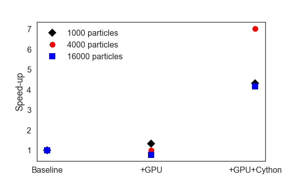
Through experimentation, we found that there was a significant amount of overhead associated with the original Python version of calculateAcceleration. Therefore, we optimized the force calculation using Cython. The speed-ups with the Cython version are shown in the Advanced Features section.


Leapfrog Algorithm

Once the forces are calculated, we use the Leapfrog Algorithm to update the positions and velocities. The Leapfrog integration algorithm is a symplectic (i.e. time-reversible) method for solving the set of differential equations given by Newton's laws:
\(v = \frac{dx}{dt}\)
\(F = m \frac{d^2x}{dt^2}\)
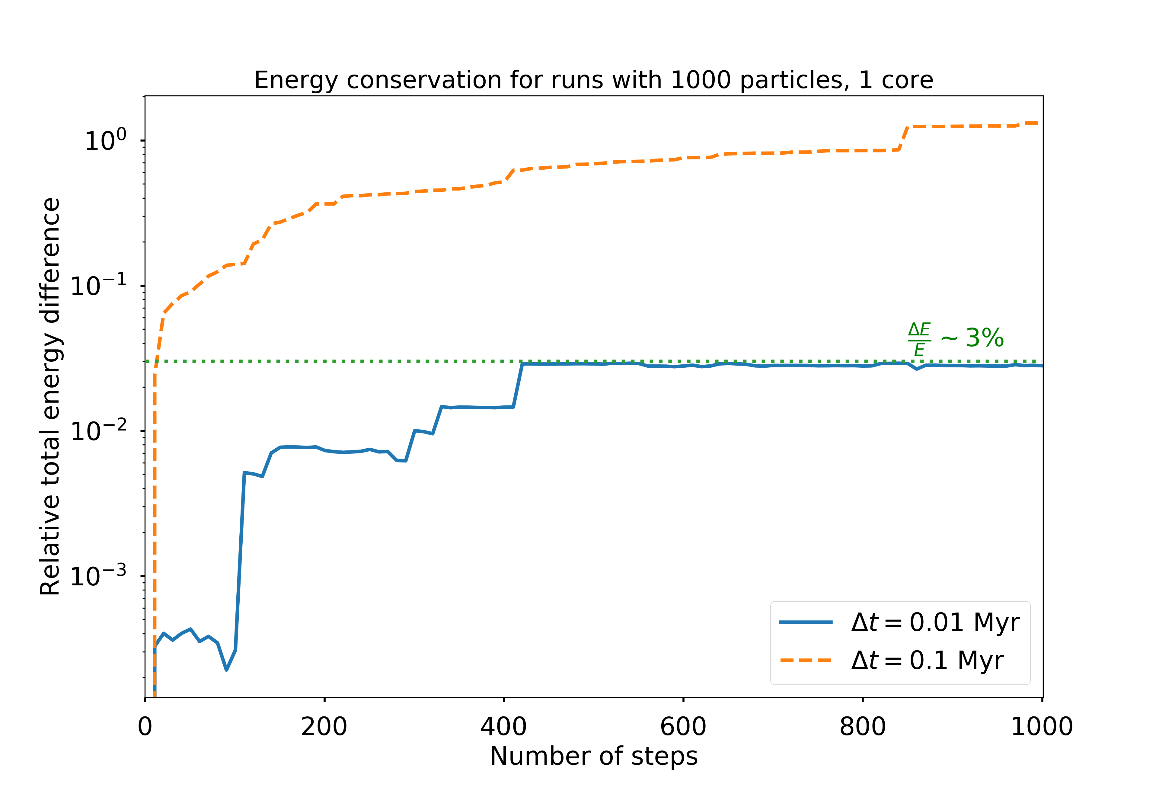
Because it is symplectic, the Leapfrog Algorithm is guaranteed to conserve energy (to reasonable precision, determined by the time step chosen). Even though it is a first-order integrator, it performs better than higher-order algorithms (like 4th order Runge-Kutta) at conserving energy over many time steps. The algorithm is nearly identical to the Euler method, except the velocities and positions are computed at half-timestep offsets: 
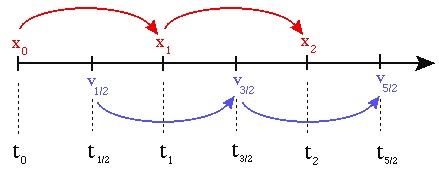
Therefore, there is an initial self-start phase of a half-step:
\(a_0 = F(x_0) / m \)
\(v_{\frac{1}{2}} = v_0 + a_0 \frac{dt}{2} \)
\(x_1 = x_0 + v_{\frac{1}{2}} dt\)
followed by the regular Euler updating kick-drift steps:
\(a_1 = F(x_1) / m \)
\(v_{\frac{3}{2}} = v_{\frac{1}{2}} + a_1 dt\)
\(x_2 = x_1 + v_{\frac{3}{2}} dt\)
We discuss the choice of timestep that results in acceptable levels of energy error below.


Parallel Algorithm

Each step of the N-body integration algorithm has the following structure:

  1. Build the Octree
  2. For each particle: compute the total force by traversing the Octree
  3. Update the velocities and positions using LeapFrog time integration algorithm
We approach the parallelization of the entire code using a hybrid approach, combining MPI and CUDA. The major limiting step is Step (1), the creation of the Octree, which is not parallelized without significant changes to the algorithm (see below for suggested improvements). Therefore, the entire catalog of simulated particles is loaded into an individual process at the beginning of each timestep, before the tree is created.

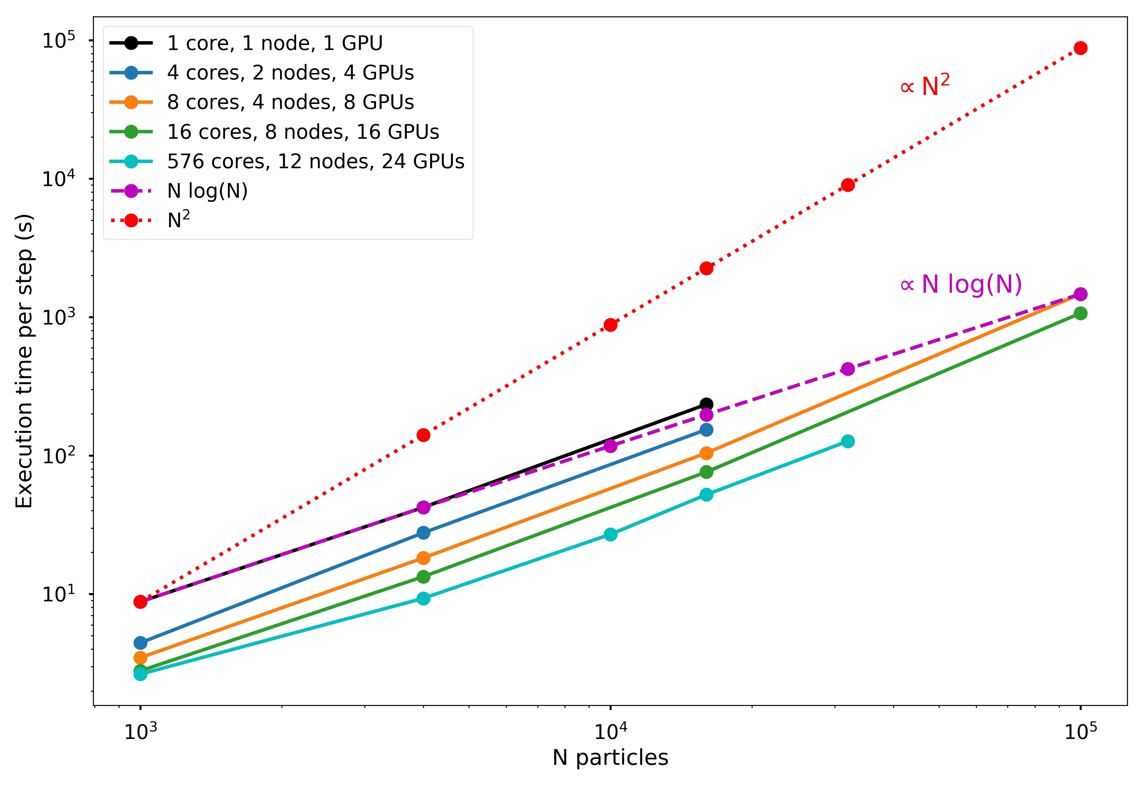
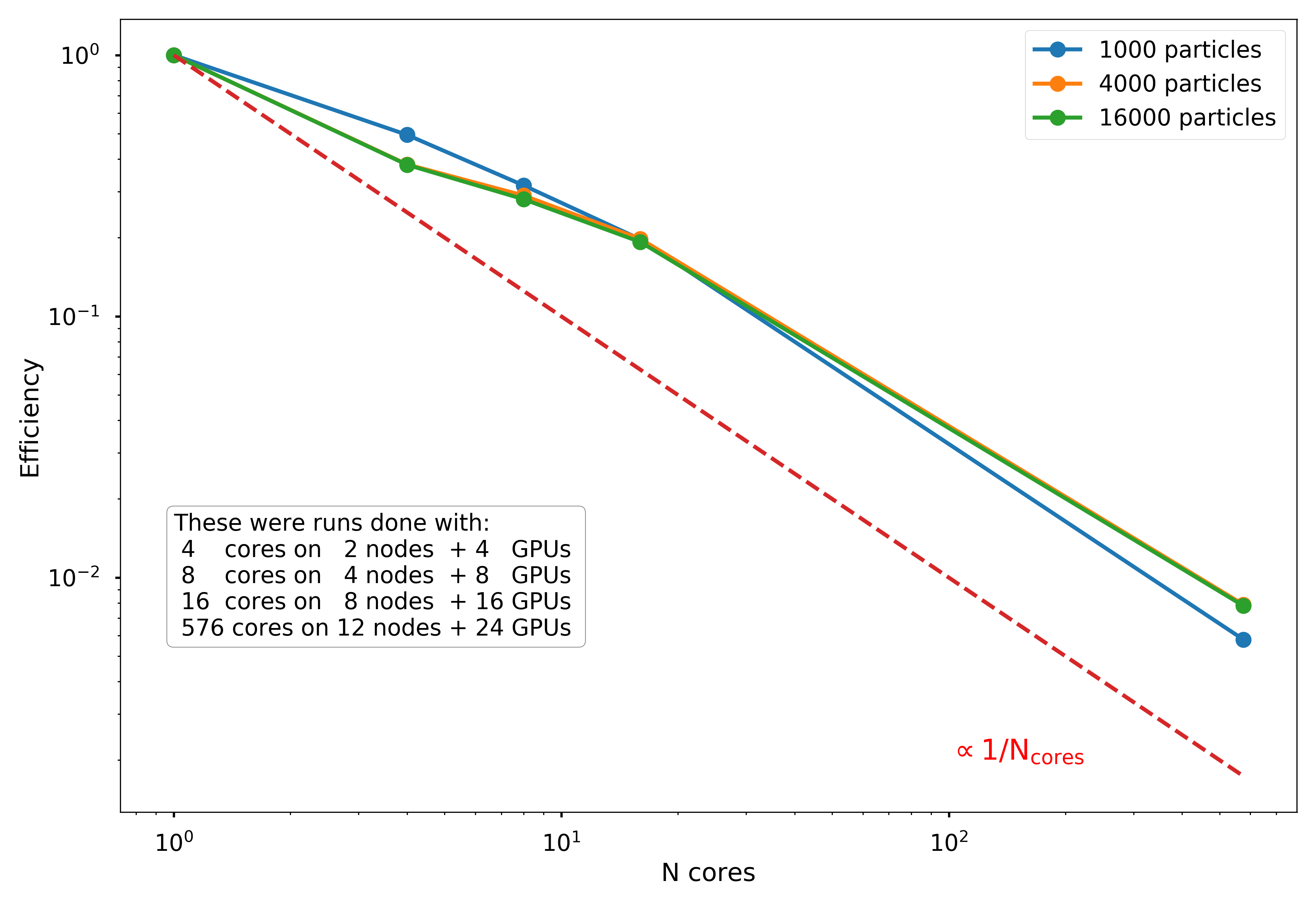
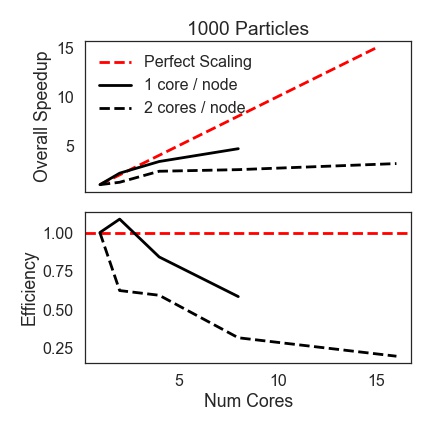
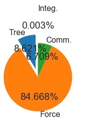
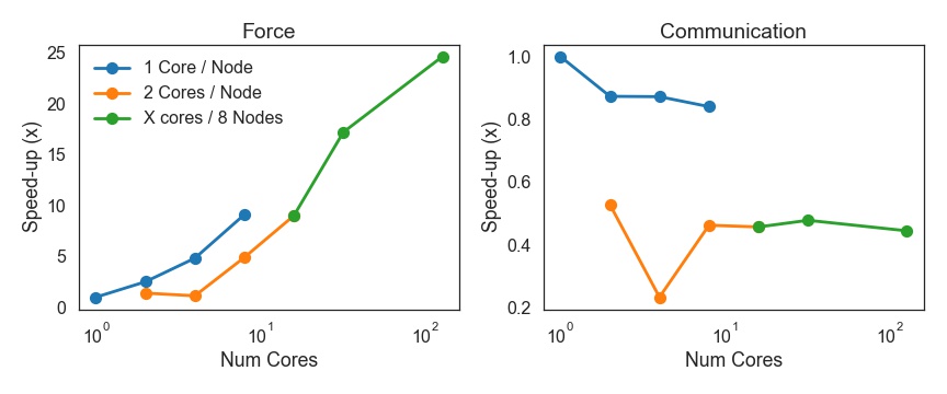
For step (2), once the tree is created, we use MPI to broadcast the entire tree to a system of distributed-memory processes. The simulated particles are then distributed nearly exactly evenly (to within \(\pm 1\) particle) across the processes, and the force calculation occurs in parallel. As discussed below, the force calculation is initially one of the most computationally demanding portions of the code, but this is conveniently the most trivially parallelizable portion, as distributing particles onto more processes nearly linearly reduces the execution time.

The second phase of parallelization comes in step (3), as we implemented the time integration step on GPUs using PyCUDA. The velocity and positions are updated for each particle in parallel on the GPU processors, which theoretically should provide significant speed-up. However, there are non-trivial overheads involved in moving to GPU acceleration. For one, the communication overhead of sending data to/from the GPU over the PCI-e bus can be significant, and speed-ups over basic Python implementation may not be seen unless a very large number of particles is used.

In addition, the number of GPUs available on a given node is typically much smaller (around 2, when available at all) than the number of CPUs. This means that for a fixed number of nodes, there may be as many as 32 times more CPUs available than GPUs. If all CPUs are being used to distribute MPI processes, then many processes will need to bind to the same GPUs, which limits the overall scalability of the GPU algorithm. In the sections below we examine these potential limitations, ultimately finding that the GPU acceleration of the time integration step does not significantly improve the execution time in our tests, likely because too few particles were used to overcome the overheads.

Including the communication overheads, the final parallel algorithm has the following steps:
  1. Build the Octree (on primary MPI node)
    • Octree is broadcast to all MPI nodes
  2. For each particle: compute the total force by traversing the Octree
    • Particle positions and velocities are distributed across MPI nodes
  3. Update the velocities and positions using LeapFrog time integration algorithm (on the GPU)
    • Particle positions, velocities, and accelerations are transferred to the GPU
    • Updated particle data retrieved from GPU
  4. Entire particle catalogs are sent back to the primary MPI node


Advanced Features

We found that a pure Python implementation of the force calculation came with many overheads due to looping in Python. Instead, we wrote a Cython version of the force calculation and traversal to mitigate this. We found that, on average, the Cython version performed three times faster than the pure Python version. As discussed later, however, the GPU acceleration was fairly insignificant, or even detrimental, as the communication overhead was simply too large for this relatively small simulation size.


Infrastructure

The BEHALF package was developed and tested in Python 3.6 (but backported to support 2.7). Serial jobs without GPU acceleration were tested on Harvard's Odyssey cluster, on a private research queue. Each core on the queue has a CPU clock of 2.3 GHz and operates on CentOS release 6.5.

The primary testing runs were performed on the holyseasgpu queue. Each of the 12 available nodes on this queue have 48 cores, a CPU clock of 2.4 GHz, and 2 NVIDIA Tesla K40m GPUs, operating on CUDA 7.5.

The BEHALF package was tested with the following Python package versions:

  • numpy: v1.12.1
  • pycuda: v2017.1.1
  • mpi4py: v2.0.0
  • future: v0.16.0
  • cython: v0.26

For details on the installation requirements and dependencies, see the Github Source Repository.


Performance and Analysis


Initial conditions - Plummer sphere

We will test our code by simulating an elliptical galaxy, modeled by the Plummer density profile.

Galaxies in our Universe come in a variety of shapes and colors, and they are often subdivided into two main classes: elliptical glaxies and spiral galaxies. The number of elliptical galaxies is higher in the densest regions of galaxy clusters, and overall, ellipticals tend to have redder colors and much lower star formation rates than spiral galaxies.

The Plummer model (Plummer 1911) was initially developed for globular star clusters, yet it is often applied to the study of elliptical galaxies due to its relatively simple form and analytic solution for the distribution function.

The Plummer 3D density profile is given by:
\(\rho(r) = \left(\frac{3M}{4\pi a^3}\right) \left( 1 + \frac{r^2}{a^2}\right)^{-5/2}\)
where M is the total mass of the galaxy, and a is the Plummer radius - a scale parameter which sets the size of the cluster core.

The mass enclosed within radius r is:
\( M(\lt r) = 4 \pi \int_0^r r^2 \rho (r) dr = M \frac{r^3}{(r^2 + a^2)^{3/2}} \)

The Plummer model has a distribution function \(f(E)\) that has an analytic expression - it is a polytrope with index \(n=5\) (see, for e.g., Binney & Tremaine 2011) and the distribution function for polytropes follows:
\(f(E) \propto |E|^{n-3/2} \Rightarrow f(E) \propto |E|^{7/2}\) for Plummer
Thus, the probability for a particle to have absolute velocity \(v\) at radius \(r\) from the center of the galaxy is:
\(g(v) dv \propto |E|^{7/2} v^2 dv \)
Letting \( x \equiv v/v_{esc}\) , where the escape velocity of a particle in the Plummer model is:
\(v_{esc} = \sqrt{\frac{2GM}{a}} \left[ 1 + \left(\frac{r}{a}\right)^2\right]^{-1/4}\)
allows us to simplify the expressions for the energy per unit mass \(E \propto (x^2 - 1)\) and the probability for a particle at radius r to have velocity v: \( g(x) \propto x^2 (1-x^2)^{7/2}\)

Based on the discussion in Aarseth et al. (1974), we use the rejection technique to generate random pairs of values \((g_0, x_0)\), where \(x_0\) is between 0 and 1 (implying initial particle velocities between 0 and \(v_{esc}\)), and the velocity probability function \(g\) is allowed to vary between 0 and \(g_{max} \simeq 0.1\). The name of the rejection technique comes from the fact that only those pairs of values for which \(g_0 \leq g(x_0)\) will be kept. This method ensures that, as long as we sample a sufficiently large number of particles, their final velocity distribution will follow \(g(x)\).

We simulated an elliptical galaxy with a total mass of \(10^{14} \mathrm{M}_\odot\) and half-mass radius of roughly 50 kpc. This elliptical galaxy is thus approximately 100 times more massive than our own Milky Way galaxy (which is a disk galaxy). Most of our test runs involve \(10^3 - 10^5\) particles, and therefore, we chose a softening length of 0.01 kpc (for more details on choosing a good softening length value, see for e.g. Athanassoula et al. 2000). We also ran tests simulating the merger between two equal mass \(10^{14} \mathrm{M}_\odot\) elliptical galaxies, which are shown in the movies section.


Physical Performance and Model Accuracy

To test the accuracy of our code, we compute the relative total energy change over a large number of time steps. The figure below shows the change in the total energy of the system with respect to the initial total energy, i.e., \((E(t)-E(t=0))/E(t=0)\), for an elliptical galaxy modeled using 1000 particles and with a total mass of \(10^{14} \mathrm{M}_\odot\). In both cases, we ran our code for 1000 time steps, but with a different time step size: 0.1 Myr shown in orange and 0.01 Myr shown in blue. We find that for a time step of 0.01 Myr, our relative total energy change saturates at the percent level, providing us with a sufficiently accurate method to run long simulations. We note that the relative error in the total energy conservation will change as a function of the time step size, the choice of softening length (which we set at 0.01 kpc in order to avoid false scatterings between particles very close to each other), and the \(\theta\) parameter for the Barnes-Hut algorithm (discussed below).

The accuracy of the Barnes-Hut algorithm is strongly related to the choice of distances over which we apply the far-field force approximation. Let's consider the distance to the center of an octree cell to be \(D\) and the width of the said cell to be \(L\). A critical parameter of the BH algorithm is \(\theta = L/D\). This is an adjustable parameter, which tells the algorithm that for particles sufficiently far away such that \(L/D \lt \theta\), those particles should be approximated by their center of mass. Naively, setting \(\theta = 0\), reduces the Barnes-Hut algorithm to an exact particle-particle force calculation, because no particles will be sufficiently far away to satisfy the requirement \(L/D \lt \theta\). As we increase \(\theta\) more and more, the algorithm speeds up significantly, yet the relative error in the force computation also increases. These trends are shown in the figure below. We ran several tests with values of \(\theta\) ranging from 0 to 2, and we decided that a value of \(\theta = 0.5\) gives us a good compromise between the running time and the force computation error (\(\sim 10^{-3}\) for \(\theta=0.5\)).

Based on the discussion above, the following simulations were run using a time step \(\Delta t = 0.01\) Myr, far-field force approximation parameter \(\theta = 0.5\), and softening length of 0.01 kpc.


Parallel Performance and Scalings


Scaling with number of cores

To begin with, we tested the performance of the BEHALF algorithm in the Strong-Scaling regime by analyzing the time taken for each time step to simulate a Plummer sphere with 1000 particles. The baseline test, run on 1 core with 1 GPU, took an average of 8.5 seconds for a timestep.

It is slightly ambiguous how to define "scaling up" the number of cores used, as there are three total dimensions of "scale-up":

Due to the architecture limitation of no more than 2 GPUs on a node, we initially tested in two scaling regimes: scaling with 1 core (hence 1 GPU) per node, and scaling with 2 cores (2 GPUs) per node. For a fixed number of cores (say, 8), this resulted in significantly different results due to the difference in communication overhead (between cores on the same node, and wrangling multiple GPUs on the same node). The plot below shows the overall speedup and scaling efficiency in these two regimes, as we scale up from 1 to 8 nodes. Very surprisingly, the efficiency is significantly better when 1 core per node is used than 2 cores. We were unable to explore this issue fully, but our suspicion is that it may have to issues with processor affinity (whether the processes are being bound on individual processors or on the same processor).

We additionally profile individual portions of the code, and how those profiles scale with number of cores. First, we show below the fraction of time spent in each portion of the code for the serial code (including GPU time integration and Cython-ized force calculation). 1000 Particle Serial Run (+GPU +Cython)

In the serial run, even after optimizing with Cython, the force calculation takes nearly 90% of the execution time. The tree construction and communication overheads account for the remainder, with time integration taking nearly zero time (reasonable for 1000 particles).


We then compare to the serial baseline for an increasing number of cores: As we scale up to 2, 4, 8, and 16 cores, the overall speedup increases to a factor of nearly 4x, with the majority of the speed-up due to the force calculation. The communication overhead increases slightly, which is to be expected. The integration time also increases slightly, likely due to overheads in communicating with multiple GPUs.
We also test how the algorithm scales when we surpass 2 cores on a node. In this scaling model, there are more processes active than GPUs available, but since the integration time is such an insignificant fraction of runtime, the overhead of having multiple processors bound to a single GPU is small. Overall, we find that the more cores used, the better the speedup of the force calculation (as shown above). Once again, there is a troubling discrepancy between 1 core per node and 2 cores per node, where distributing, for example, 8 cores across 8 nodes is faster even at computing forces than distributing across fewer nodes. The communication overhead is likewise much larger for multiple cores per node, which seems unusual for MPI.

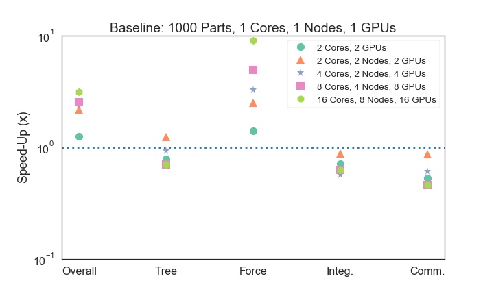
1000 Particle Run, 16 cores, 8 nodes(+GPU +Cython)

Finally, we show the timing profile for a scaled-up run with 16 total cores (and 16 GPUs) spread across 8 nodes. Once scaled up to 16 cores, the force computation takes only around 30% of the execution time, while the communication overhead and tree construction have balooned to each encompass 30% and 40% (respectively) of the execution time.


Scalings with the number of particles

The figure below shows the scaling between the median time step of our BH code and the total number of particles in the simulation. We are showing a range of tests with 2 cores per node and 2 GPUs per node, with the total number of particles being [1000, 4000, 10000, 16000, 100000]. We also include for comparison, serial runs shown in black, and in light blue we show our results when utilizing the maximum number of cores (576) and GPUs (24) available on the holyseasgpu queue on Odyssey. The dotted red line shows the \(N^2\) scaling expected for an exact particle-particle force calculation, while the dashed magenta line indicates the theoretical \(N \,\mathrm{log}(N)\) expectation for the Barnes-Hut octree implementation. Our implementation matches \(N \,\mathrm{log}(N)\) very well for particle numbers up to \(\sim 2\times 10^4\). For larger simulations, our scaling gets slightly worse than \(N \,\mathrm{log}(N)\) (but still much better than \(N^2\)) because the depth of the tree can increase rapidly due to false scatterings between particles. As two particles get close together, the very large gravitational force between them multiplied by our fixed time step will lead to an artificially large scatter, causing one of the particles to be flung far away from the center of the simulation box. In order to accommodate this particle, the tree traversal will start to take longer than the average \(\log(N)\) number of operations.

We also examine how the efficiency changes as a function of number of particles, i.e. in the weak-scaling regime. The iso-efficiency curve will be very flat, as there is only a small difference in efficiency at much larger simulation sizes. This implies that the iso-efficiency scaling of the algorithm is fairly weak, as a small increase in the number of processors requires a large increase in problem size in order to retain constant efficiency.

Results and Conclusions


Resulting Movies

Below are two movies exmplifying the type of simulation runs we tested in our project. These are showing the evolution of (1) a \(10^{14} \mathrm{M}_\odot\) elliptical galaxy and (2) the merger between two \(10^{14} \mathrm{M}_\odot\) galaxies, using our parallel implementation of the Barnes-Hut algorithm.

A movie of the projected density in the x-y plane of a 10,000 particle simulation.

A movie of a merger of two Plummer sphere galaxies (1000 particles each) in the x-y plane, applying a Gaussian smoothing kernel.


Future work

There are many avenues for improving the execution time of the force calculation. Below we list a few such directions, in order of increasing difficulty and potential improvement:

Cythonize the entire tree data structure
The octree structure is constructed in Python, and while Cython allowed us to improve speed in traversing the tree for force calculations, there were still significant overheads involved in calling Python object features from the Cython code. If the entire octree creation were re-written in Cython, such that there was no Python overhead involved, we anticipate a speed-up of around 50% to 2x in the tree-construction and force calculation phases.

Use kD trees instead of octree
K-Dimensional trees are significantly more memory-efficient, and would decrease the overhead in traversing the tree and broadcasting it to all nodes. The construction of kD trees is also more easily parallelizable than Octrees.

Use GPUs to do force calculations
Optimizing the force calculations further could involve transferring the trees to the GPU, and then computing particle forces in parallel on the GPU. The many-core nature of the GPU could improve the throughput significantly, although the overhead of transferring the tree across the data bus would need to be considered.

Partially Cache the Octree
Depending on the size of the timestep, many particles do not move very far each iteration, meaning that the Octree is likely very similar from one timestep to the next. Saving the Octree and only updating portions that have changed significantly could reduce the tree construction time significantly.

Parallelize tree construction
Besides MPI communication, the primary serial component of our code is the computation of the tree, which naiively requires one node to have all particles stored in memory. An advanced implementation of the algorithm could construct the tree in parallel, perhaps by assigning the first 1 or 2 levels of the sub-tree to different processes, and ensuring that nearby particles are assigned to similar nodes. More MPI communication would be required in the force computation, in the cases where particles nearby to box boundaries would need to traverse neighboring portions of the overall tree.

References

  • Aarseth S. J., Henon M., Wielen R., 1974, A&A, 37, 183
  • Angulo, R. E., et al. "Scaling relations for galaxy clusters in the Millennium-XXL simulation." Monthly Notices of the Royal Astronomical Society 426.3 (2012): 2046-2062.
  • Athanassoula, E., et al. “Optimal softening for force calculations in collisionless N-body simulations.” Monthly Notices of the Royal Astronomical Society 314.3 (2000): 475-488.
  • Barnes, Josh, and Piet Hut. "A hierarchical O (N log N) force-calculation algorithm." nature 324.6096 (1986): 446.
  • Brož, Miroslav, and David Vokrouhlický. "Asteroid families in the first-order resonances with Jupiter." Monthly Notices of the Royal Astronomical Society 390.2 (2008): 715-732.
  • Binney J., Tremaine S., 2011, Galactic Dynamics. Princeton University Press
  • Darden, Tom, Darrin York, and Lee Pedersen. "Particle mesh Ewald: An N⋅ log (N) method for Ewald sums in large systems." The Journal of chemical physics 98.12 (1993): 10089-10092.
  • Katz, Neal, David H. Weinberg, and Lars Hernquist. "Cosmological simulations with TreeSPH." arXiv preprint astro-ph/9509107 (1995).
  • Newton, Isaac. "Principia mathematica." Isaac Newton’s Philosophiae Naturalis Principia Mathematica, Harvard University Press, Cambridge, MA (1972).
  • Plummer H. C., 1911, MNRAS, 71, 460
  • Springel, Volker. "The cosmological simulation code GADGET-2." Monthly notices of the royal astronomical society 364.4 (2005): 1105-1134.
  • Wadsley, James W., Joachim Stadel, and Thomas Quinn. "Gasoline: a flexible, parallel implementation of TreeSPH." New Astronomy 9.2 (2004): 137-158.